Orbital Adjustment for Normal Point Formation
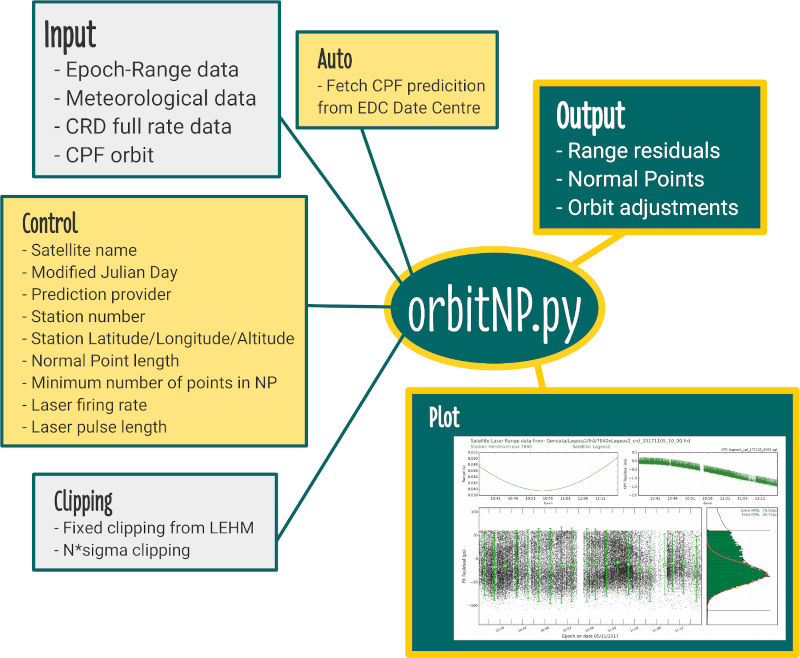
The orbitNP.py software program processes Satellite Laser Ranging (SLR) observations and calculates orbital corrections to flatten range residuals so that normal points may be calculated.
The code is written in Python3 and has its origins in legacy FORTRAN code developed at the Space Geodesy Facility, Herstmonceux, UK. In 2018, it was made freely available, with this disclaimer, to download for the SLR community.
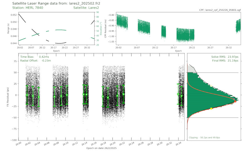
orbitNp.py takes in epochs and 2-way time-of-flight intervals recorded during a SLR pass and produces flattened observed-computed (O-C) residuals.
It uses a corresponding ILRS CPF prediction file that covers the observation time period to produce range residuals. Radial offset and time bias corrections to the orbit are solved for through an iterative least squares process to flatten the residuals. These flattened residuals can then be averaged in bins and time stamped to form precise range observations called normal points.
The epochs and ranges can be supplied in the form of pre-processed SLR returns in ILRS full-rate CRD data files which can be quickly examined for a particular station and satellite.
Alternatively, raw epoch-range data can be processed. Correction delays, such as those required for optical filters, must be pre-applied. Similarly, any epoch corrections must be applied to refer the recorded epoch to the SLR reference point. The data should contain satellite track with only a small range window of surrounding noise. System delay calibration and local meteorological data must also be provided.
Meteorological data (Temperature, Pressure and Humidity) recorded at the SLR station is required to correct for delays through the atmosphere, using the Marini-Murray model. This is taken from the full-rate CRD file or must be provided separately.
The latitude, longitude and altitude of the SLR station are required. These can be entered or SLR station coordinates can be taken a SINEX file (found here on CDDIS (EARTHDATA login required)).
The program can output files that contain:
- Normal points in CRD format.
- Full-rate data in CRD format. This can include surrounding data not used in the noraml point calculation, indicated using the filter flag.
- Range residuals with epochs.
- Orbit correction parameters from the solution.
###
# Update History
###
Version 1.3
- Include CDDIS as a source for automatic cpf predictions and crd downloads. EARTHDATA login details requested and stored locally in .earthda talogin file.
- Attempt to download fr2 full-rate file from Data Center if does not exist on drive.
- Downloads CDDIS full-rate data files that are gzipped.
- Clipping varies depending on the incident angle for GNSS flat LRA. This results in realtively wider acceptance at low elevations.
- Jpeg output option.
- Read and output receive amplitude records.
- Allow dynamic axes labelling for matplotlib plots.
- Specify output folder name to save plots.
Version 1.2.2
- Changes made to remove Linux commands so that orbitNP.py could be run on Windows.The 'wget' command is still required and this is available to download and put in the orbitNP folder.
- Option to keep open the matplotlib plot window and block the program from completing.
- Output clipping parameters to file clip.out
Version 1.2.1
- CPF interpolation replaced with high order polynomial fit. This is to provide better prediciton values and to remove some actifacts in range residuals.
- Update matplotlib subplot axis referencing method to work with the latest versions.
Version 1.2
- Gauss fit filter added.
- Peak-Mean default as 1*sigma iterative mean.
- Option to calculate a '50' record if not included in full-rate CRD file.
- Include option to output final ranges in CRD format with met and calibration values.
- Filtering at two levels. The first is to form the normal points and the second is to include in the full-rate output.
- Include option to input satellite centre of mass offset to improve the orbit solution and flatten range residuals.
- Indicate if individual normal point residual bins have slopes.
- Select SLR station data in full-rate data file from list.
- Matplotlib figure window now kept open to allow for much faster plotting of a series of passes.
Version 1.1
- Added import of warnings Python3 module
- New method for cal2mjd() and mjd2cal()
- Include option for full CRD normal point output file.
- Include 1st iteration quick-pass option to prevent high density segments dominating pass fit.
- Include input of 'System Configuration ID'.
- Adjusted method for gauss fit to front of residual distribution.
- Allow for disagreement in first epoch and H4 record.
- Station coordinates and velocities taken from an ILRS SINEX solution file.
- Peak-Mean calculated using a tangent fit to a smoothed profile.
- Option to include unfiltered range measurements


