GNSS analysis
Site coordinate and baseline determination provides local stability information and results for comparison with the other independent co-located techniques.
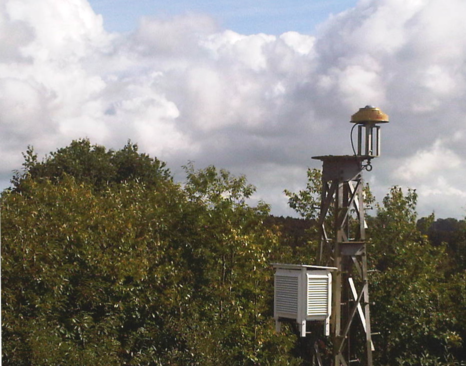 The SGF IGS GNSS sites, HERS and HERT track GPS and GLONASS satellites and send data daily and hourly to the International GNSS Service (IGS).
HERS was installed in 1992 and is in close proximity to both the SLR and absolute gravimeter locations. HERT began collecting data in 2003.
The SGF IGS GNSS sites, HERS and HERT track GPS and GLONASS satellites and send data daily and hourly to the International GNSS Service (IGS).
HERS was installed in 1992 and is in close proximity to both the SLR and absolute gravimeter locations. HERT began collecting data in 2003. GNSS analysis at the SGF uses the GAMIT/GLOBK GPS analysis package, which was developed by Massachusetts Institute of Technology, Scripps Institution of Oceanography, and Harvard University.
GAMIT can calculate high quality co-ordinate solutions for the SGF sites in a network of other GNSS sites using satellite orbits, Earth orientation parameters and antenna phase centre offsets. The SGF analysis uses an ionosphere-free linear combination of the L1 and L2 frequencies and automatically resolves phase ambiguities in the data using the pseudo-ranges. The output from this option provides a characterisation of station performance, which is used to re-weight the data from each station. It is necessary to tightly constrain UT1 because it cannot be resolved independently from GNSS satellite parameters. And the other EOPs are also constrained to their International Earth Rotation and Reference Systems Service (IERS) values and the satellite orbits were constrained to the 'final' orbits from the IGS.
 The phase centre offsets for both the ground and satellite antennas are provided as absolute values.
GAMIT applies an ocean tide model from an interpolated grid.
Likewise, an atmospheric loading model can be applied.
The GAMIT results are 'stabilised' onto the The International Terrestrial Reference Frame (ITRF) using the GLOBK package.
The phase centre offsets for both the ground and satellite antennas are provided as absolute values.
GAMIT applies an ocean tide model from an interpolated grid.
Likewise, an atmospheric loading model can be applied.
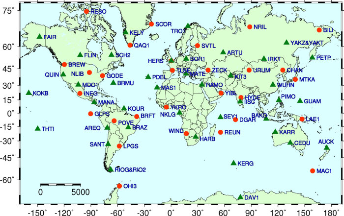
The GAMIT results are 'stabilised' onto the The International Terrestrial Reference Frame (ITRF) using the GLOBK package.The sites were chosen to achieve global coverage and can be seen on the map to the right. The analysis was done in two global networks to aid the processing required, which were combined at a later stage. A global network was used, rather than a regional network, in order to apply the least constraints to the coordinates of the SGF sites.
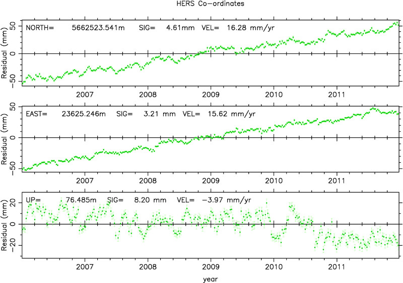
The time series below shows the North, East and Up co-ordinates from this analysis for the HERS site. The drift North and East is clear due to the movement of the European plate and height variations are seen at the level of a few centimetres.
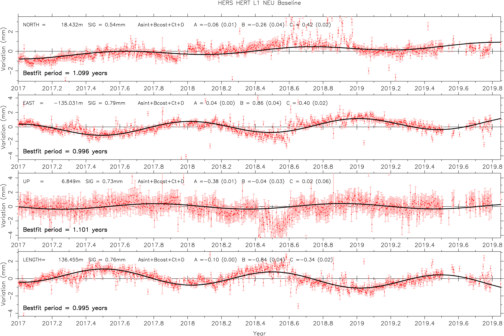
The differential baseline vector components from HERS to HERT are plotted below: