


During a Starlette pass on Sept 28th the observer made a mistake and put in an offset which caused the track to get too close to the point that the C-SPAD was armed. After a minute or so he realised this and corrected the offset so that the track was greater than 50ns after arming the C-SPAD.
|
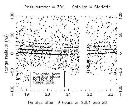
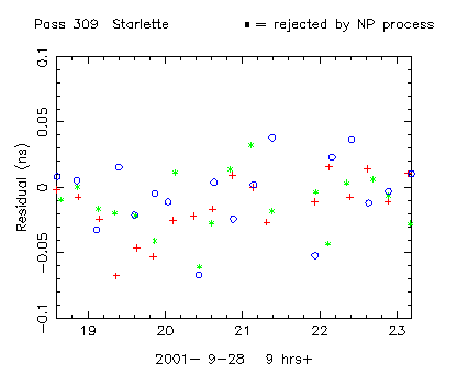
Figure 1. Expanded plot of the raw residuals for the whole pass showing the semi-train and noise. Outside minutes 19.2 and 21 noise can be seen greater than 50ns below the track. The gap in tha data during minute 22 is when the satellite went close to the Sun. |
The pass looks quite normal and was reduced by our standard procedures. As
part of our processing we insist that the final data set fit various
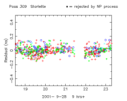
constraints. This data set failed with a value for the Peak-LEHM (as
derived from the Gaussian distribution process DISTRIB - SLRMAIL 0008)
outside limits defined by the Herstmonceux system. As our system is strict
the software will not let you send out data which fails any test. The
observer must therefore find out why the data has failed.
|
Figure 2. Plot of the final residuals. The different coloured points represent the different pulses in the semi-train. There is a clear "bump" through minute 19 |
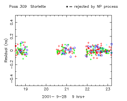
After some investigation it was realised that the observer had made a mistake during the observing. The pass was then re-reduced with all possible offending data removed.
|
Figure 3. Final residuals with offending data missing. Note that the data for minute 23 has now come back in line. |
|
|
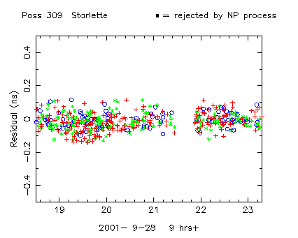
Figure 4b shows the mean values of the residuals for each pulse for
each normal point bin.
From Figure 1 we can see that the C-SPAD was armed between 30ns and 50ns before the track for the erroneous data although the exact value is uncertain. The error values for the uncompensated channel obtained from calibrations as shown in Figure 5 for pre-arming values of 30ns-50ns agree closely to those shown in Figure 4b.
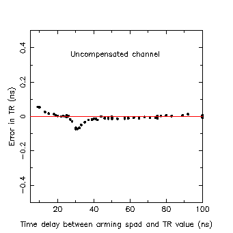
Figure 5 |
A series of local target observations were made each using different
delays between the time of arming the C-SPAD and the calibration. The
data for each calibration was then compared with a "control" calibration
taken with a delay of 100ns between arming and data returns. To give us a
fuller data set we used data from the first four pulses of our semi-train.
Figure 5 shows the results for the uncompensated channel of the C-SPAD. |
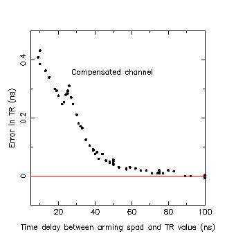
Figure 6 |
Figure 6 shows the results for the compensated channel of the C-SPAD.
It can be clearly seen that the behaviour of the compensated and uncompensated channels are considerably different and that much larger errors are introduced if you get too close to the arming point for the C-SPAD. |